Individual Storm Analysis

This sample script illustrates how to retrieve a single storm from the HURDAT2 dataset, and make plots and analyses of this storm.

import tropycal.tracks as tracks
import datetime as dt

HURTDAT2 Dataset

Let’s start by creating an instance of a TrackDataset object. By default, this reads in the HURDAT2 dataset from the National Hurricane Center (NHC) website. For this example we’ll be using the HURDAT2 dataset over the North Atlantic basin.

HURDAT data is not available for the most recent hurricane seasons. To include the latest data up through today, the “include_btk” flag would need to be set to True, which reads in preliminary best track data from the NHC website.

hurdat_atl = tracks.TrackDataset(basin='north_atlantic',source='hurdat',include_btk=False)

Individual storm analysis

Individual storms can be retrieved from the dataset by calling the get_storm() function, which returns an instance of a Storm object. This can be done by either entering a tuple containing the storm name and year, or by the standard tropical cyclone ID (e.g., “AL012019”).

Let’s retrieve an instance of Hurricane Michael from 2018:

storm = hurdat_atl.get_storm(('michael',2018))

This instance of Storm contains several methods that return the storm data back in different data types. The following examples will show how to retrieve 3 different data types.

Retrieve a dictionary of Michael’s data:

storm.to_dict()

Retrieve xarray Dataset object with Michael’s data:

storm.to_xarray()

Retrieve pandas DataFrame object with Michael’s data:

storm.to_dataframe()

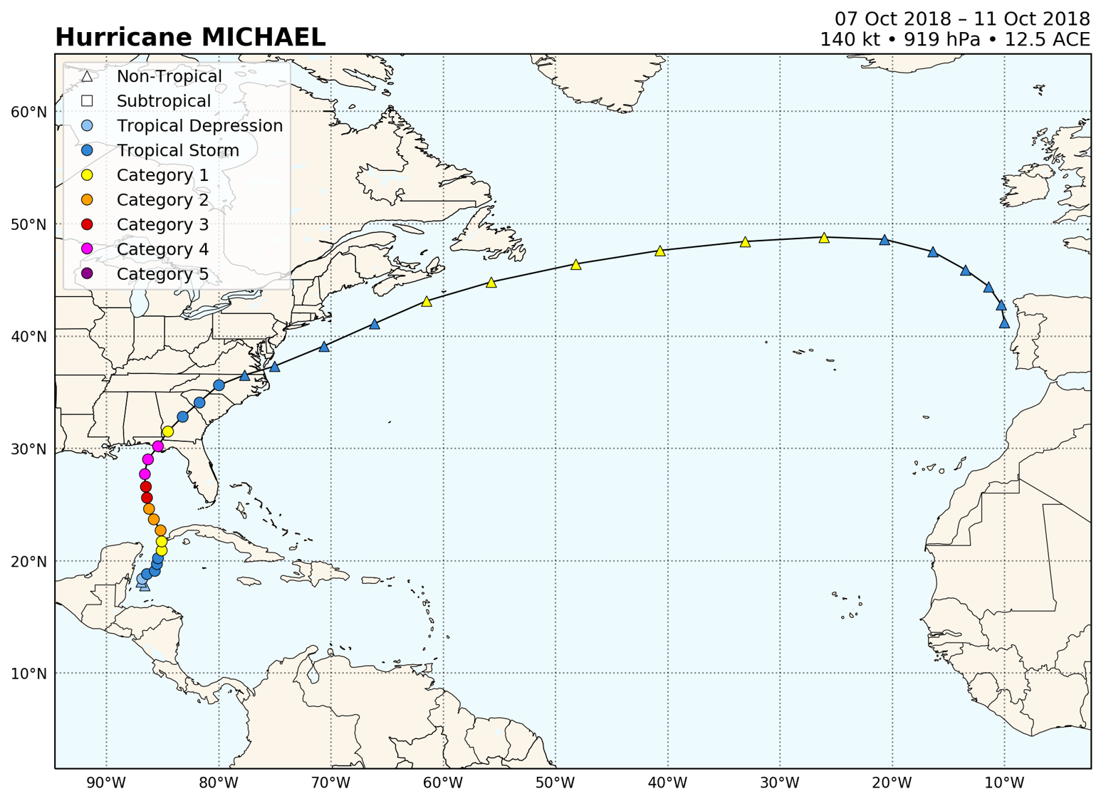
Visualize Michael’s observed track with the “plot” function:

Note that you can pass various arguments to the plot function, such as customizing the map and track aspects. The only cartopy projection currently offered is PlateCarree. Read through the documentation for more customization options.

storm.plot()

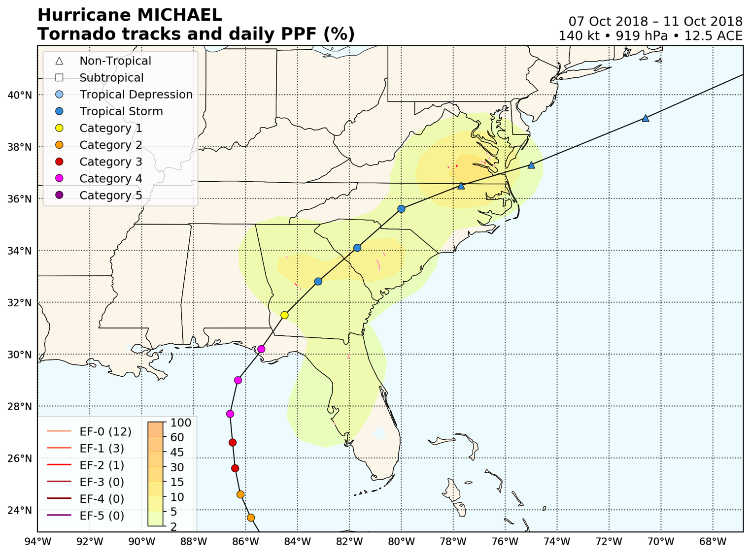
Plot the tornado tracks associated with Michael, along with the accompanying daily practically perfect forecast (PPF):

storm.plot_tors(plotPPF=True)

If this storm was ever in NHC’s area of responsibility, you can retrieve operational NHC forecast data for this event provided it is available. Forecast discussions date back to 1992, and forecast tracks date back to 1954.

Retrieve a single forecast discussion for Michael:

#Method 1: Specify date closest to desired discussion
disco = storm.get_nhc_discussion(forecast=dt.datetime(2018,10,7,0))
print(disco['text'])

#Method 2: Specify forecast discussion ID
disco = storm.get_nhc_discussion(forecast=2)
#print(disco['text']) printing this would show the same output

ZCZC MIATCDAT4 ALL
TTAA00 KNHC DDHHMM

Potential Tropical Cyclone Fourteen Discussion Number   2
NWS National Hurricane Center Miami FL       AL142018
1000 PM CDT Sat Oct 06 2018

The cloud pattern has improved in organization and surface pressures
are gradually falling, but there is no evidence that the system is
a tropical cyclone at this time.  All indications are, however, that
a tropical depression will likely form at any time soon. Strong wind
shear is expected to affect the disturbance, and the SHIPS model
only show a modest strengthening. This is in contrast to some global
models and the HWRF, which are more aggressive in developing this
system.  Since the environment is marginally favorable, the NHC
forecast only gradually strengthens the system at the rate of the
intensity consensus IVCN.  However, the forecast is highly uncertain
given the solution of the global models.

Since the system does not have a well-defined center, the initial
motion is also uncertain. The best estimate is toward the north or
360 degrees at 6 kt. Over the next 2 or 3 days, the cyclone will be
embedded within the deep southerly flow between a strong subtropical
ridge over the western Atlantic and a sharp mid-latitude trough
advancing eastward over the United States.  This flow pattern will
force the system to move northward at 5 to 10 kt across the
eastern Gulf of Mexico for the next 2 to 3 days. By day 4, the
system should have moved inland and be weakening. It should
then race northeastward farther inland across the eastern U.S.  The
track guidance envelope is remarkably quite tight. This increases
the confidence in the track forecast primarily after the cyclone
forms.

Key Messages for Potential Tropical Cyclone Fourteen:

1.  This system is producing heavy rainfall and flash flooding over
portions of Central America, and these rains will spread over
western Cuba and the northeastern Yucatan Peninsula of Mexico during
the next couple of days.

2.  The system is forecast to become a tropical storm by late
Sunday, and tropical storm conditions are expected over portions of
western Cuba, where a Tropical Storm Warning is in effect.

3.  The system could bring storm surge, rainfall, and wind impacts
to portions of the northern Gulf Coast by mid-week, although it is
too soon to specify the exact location and magnitude of these
impacts.  Residents in these areas should monitor the progress of
this system.


FORECAST POSITIONS AND MAX WINDS

INIT  07/0300Z 18.8N  86.6W   25 KT  30 MPH...POTENTIAL TROP CYCLONE
 12H  07/1200Z 19.5N  86.5W   30 KT  35 MPH...TROPICAL CYCLONE
 24H  08/0000Z 21.0N  86.2W   35 KT  40 MPH
 36H  08/1200Z 22.3N  86.1W   40 KT  45 MPH
 48H  09/0000Z 23.8N  86.3W   45 KT  50 MPH
 72H  10/0000Z 27.4N  87.2W   55 KT  65 MPH
 96H  11/0000Z 32.0N  85.0W   30 KT  35 MPH...INLAND
120H  12/0000Z 38.5N  77.5W   30 KT  35 MPH...INLAND

$$
Forecaster Avila

NNNN

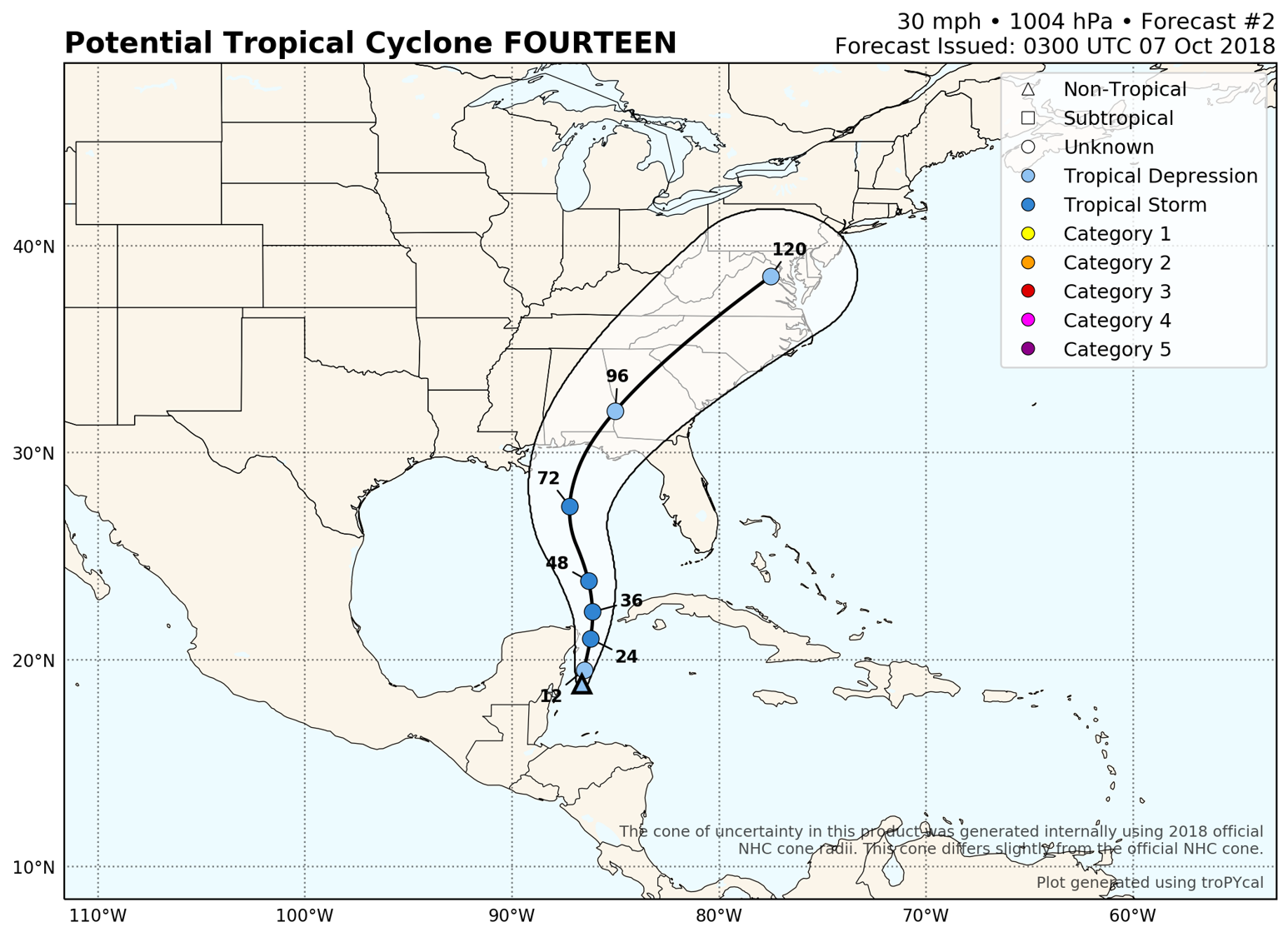
NHC also archives forecast tracks, albeit in a different format than the official advisory data, so the operational forecast IDs here differ from the discussion IDs. As such, the forecast cone is not directly retrieved from NHC, but is generated using an algorithm that yields a cone closely resembling the official NHC cone.

Let’s plot Michael’s second forecast cone:

storm.plot_nhc_forecast(forecast=2)

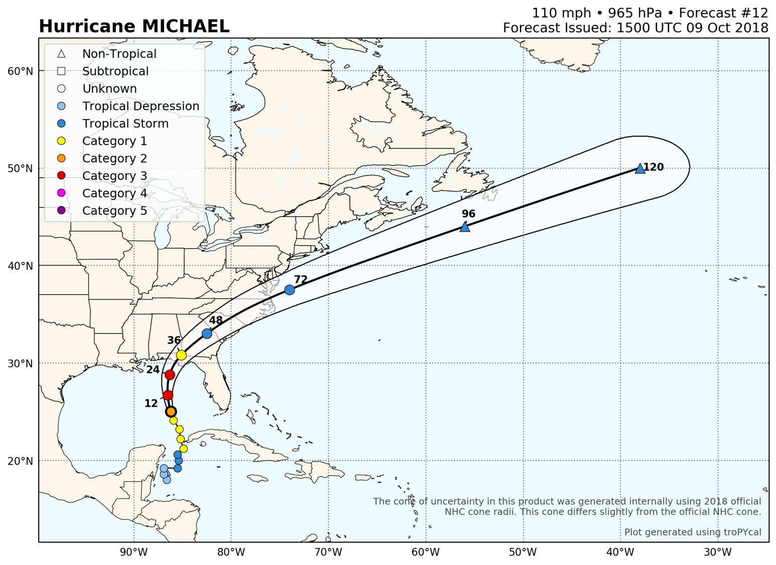
Now let’s look at the 12th forecast for Michael.

Note that the observed track here differs from the HURDAT2 track plotted previously! This is because this plot displays the operationally analyzed location and intensity, rather than the post-storm analysis data. This is done to account for differences between HURDAT2 and operational data.

storm.plot_nhc_forecast(forecast=12)

IBTrACS Dataset

We can also read in IBTrACS data and use it the same way as we would use HURDAT2 data. There are caveats to using IBTrACS data, however, which are described more in depth in the Data Sources page. We’ll retrieve the global IBTrACS dataset, using the Joint Typhoon Warning Center (JTWC) data, modified with the Neumann reanalysis for southern hemisphere storms, and including a special reanalysis for Cyclone Catarina (2004) in Brazil.

Warning

By default, IBTrACS data is read in from an online source. If you’re reading in the global IBTrACS dataset, this could be quite slow. For global IBTrACS, it is recommended to have the CSV file saved locally (link to data), then set the flag ibtracs_url="local_path".

ibtracs = tracks.TrackDataset(basin='all',source='ibtracs',ibtracs_mode='jtwc_neumann',catarina=True)

The functionality for handling storms in IBTrACS is the same as with using HURDAT2, the only limitation being no NHC and operational model data can be accessed when using IBTrACS as the data source.

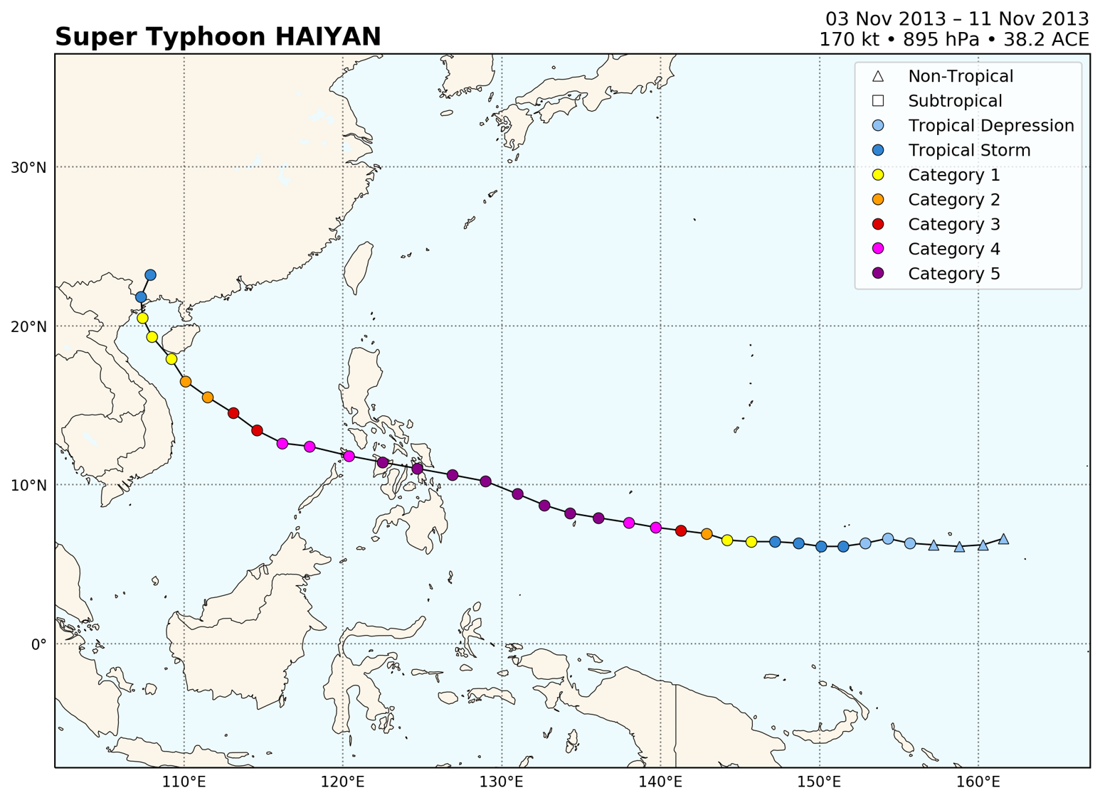
Super Typhoon Haiyan (2013) was a catastrophic storm in the West Pacific basin, having made landfall in the Philippines. With estimated sustained winds of 195 mph (170 kt), it is among one of the most powerful tropical cyclones in recorded history. We can illustrate this by making a plot of Haiyan’s observed track and intensity, from JTWC data:

storm = ibtracs.get_storm(('haiyan',2013))
storm.plot()

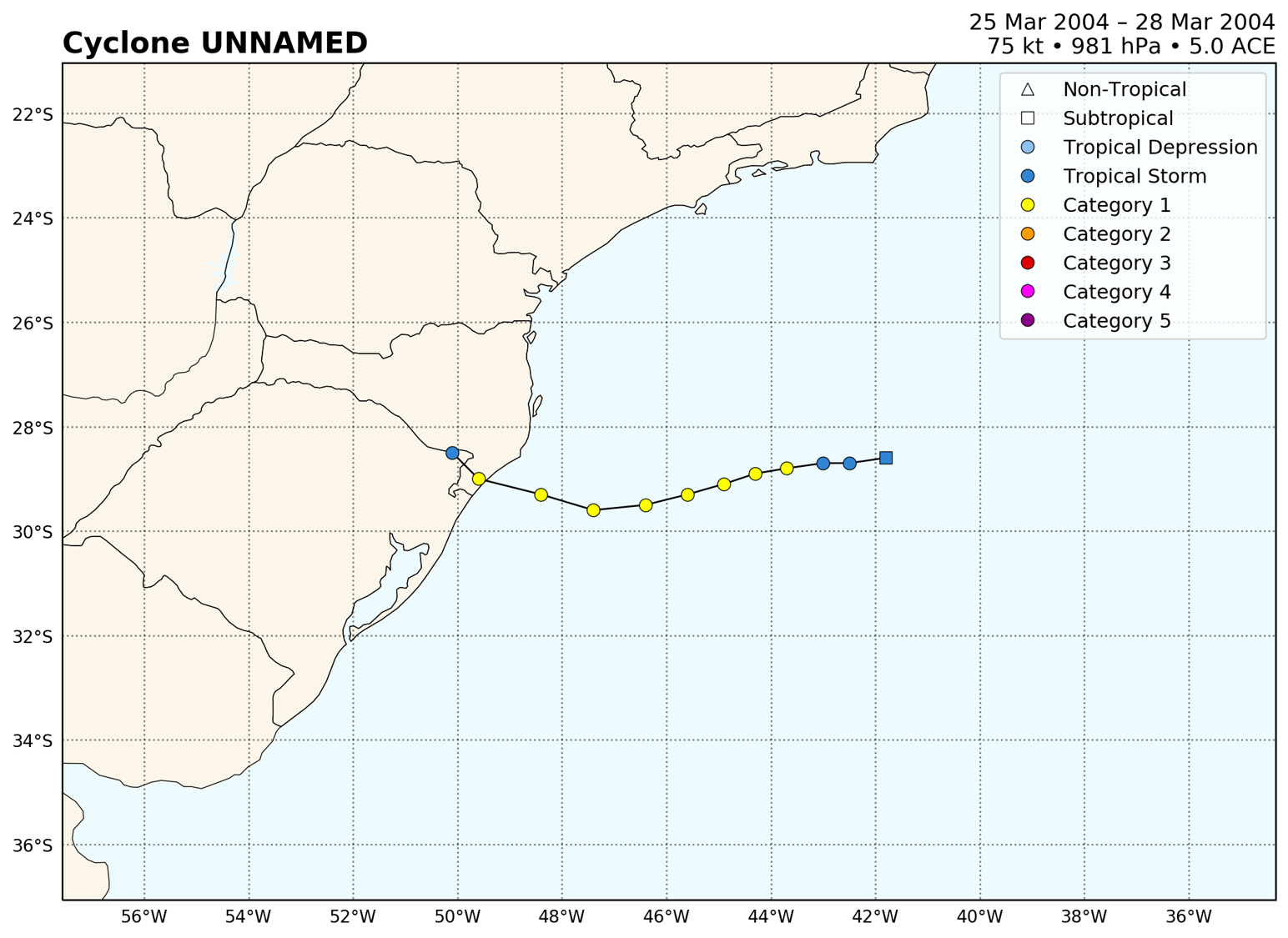
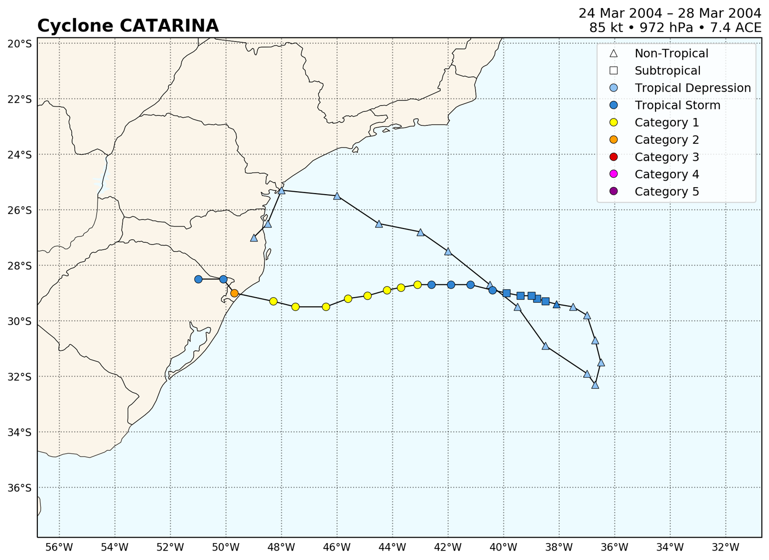
Cyclone Catarina (2004) was an extremely rare hurricane-force tropical cyclone that developed in the South Atlantic basin, which normally doesn’t see tropical cyclone activity, and subsequently made landfall in Brazil. The “Catarina” name is unofficial; it was not assigned a name in real time, and JTWC assigned it the ID “AL502004”. Recall that when reading in the IBTrACS dataset previously, we set Catarina=True. This read in data for Cyclone Catarina from a special post-storm reanalysis from McTaggart-Cowan et al. (2006). Let’s make a plot of Catarina’s observed track and intensity per this reanalysis:

storm = ibtracs.get_storm(('catarina',2004))
storm.plot()

If we were to read in IBTrACS without setting Catarina=True (which sets it to False by default) and plot the track for “AL502004”, we would get the following:

storm = ibtracs.get_storm('AL502004')
storm.plot()