Standalone Cartopy Functionality

This sample script illustrates how to leverage Tropycal’s standalone Cartopy functionality alongside its existing data structures to make custom plots and analyses.

import datetime as dt
from tropycal import tracks, utils
import cartopy.crs as ccrs
import cartopy.feature as cfeature
import matplotlib.pyplot as plt

Reading In HURTDAT2 Dataset

Let’s start with the HURDAT2 dataset by loading it into memory. By default, this reads in the HURDAT dataset from the National Hurricane Center (NHC) website, unless you specify a local file path using either atlantic_url for the North Atlantic basin on pacific_url for the East & Central Pacific basin.

HURDAT data is not available for the current year. To include the latest data up through today, the “include_btk” flag needs to be set to True, which reads in preliminary best track data from the NHC website. For this example, we’ll set this to False.

Let’s create an instance of a TrackDataset object, which will store the North Atlantic HURDAT2 dataset in memory. Once we have this we can use its methods for various types of analyses.

basin = tracks.TrackDataset(basin='north_atlantic',include_btk=False)

--> Starting to read in HURDAT2 data
--> Completed reading in HURDAT2 data (24.38 seconds)

Reading in storm data

Individual storms can be retrieved from the dataset by calling the get_storm() function, which returns an instance of a Storm object. This can be done by either entering a tuple containing the storm name and year, or by the standard tropical cyclone ID (e.g., “AL012019”).

Let’s retrieve an instance of Hurricane Michael from 2018:

storm = basin.get_storm(('michael',2018))

We now have a Storm object, containing information about its track and intensity data, as well as various methods for subsetting and analyzing it.

print(storm)

<tropycal.tracks.Storm>
Storm Summary:
    Maximum Wind:      140 knots
    Minimum Pressure:  919 hPa
    Start Time:        0600 UTC 07 October 2018
    End Time:          1800 UTC 11 October 2018

Variables:
    time        (datetime) [2018-10-06 18:00:00 .... 2018-10-15 18:00:00]
    extra_obs   (int64) [0 .... 0]
    special     (str) [ .... ]
    type        (str) [LO .... EX]
    lat         (float64) [17.8 .... 41.2]
    lon         (float64) [-86.6 .... -10.0]
    vmax        (int64) [25 .... 35]
    mslp        (int64) [1006 .... 1001]
    wmo_basin   (str) [north_atlantic .... north_atlantic]

More Information:
    id:              AL142018
    operational_id:  AL142018
    name:            MICHAEL
    year:            2018
    season:          2018
    basin:           north_atlantic
    source_info:     NHC Hurricane Database
    source:          hurdat
    ace:             12.5
    realtime:        False
    invest:          False
    subset:          False

Basic Cartopy plot

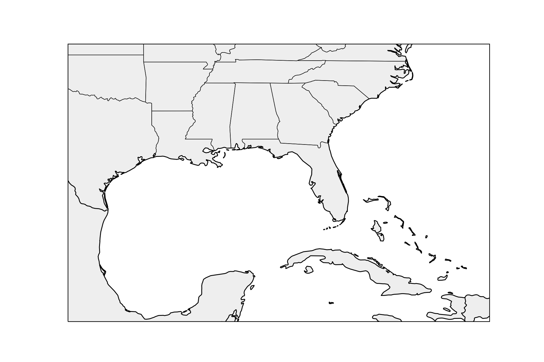
Let’s make a basic Cartopy map focused over the Gulf of Mexico, with geographic boundaries denoted and land filled in light gray. We’ll add Cartopy utility to this plot in later steps.

# Create a PlateCarree Cartopy projection
proj = ccrs.PlateCarree()

# Create an instance of figure and axes
fig = plt.figure(figsize=(9,6),dpi=200)
ax = plt.axes(projection=proj)

# Plot coastlines and political boundaries
ax.add_feature(cfeature.STATES.with_scale('50m'), linewidths=0.5, linestyle='solid', edgecolor='k')
ax.add_feature(cfeature.BORDERS.with_scale('50m'), linewidths=1.0, linestyle='solid', edgecolor='k')
ax.add_feature(cfeature.COASTLINE.with_scale('50m'), linewidths=1.0, linestyle='solid', edgecolor='k')

# Fill in continents in light gray
ax.add_feature(cfeature.LAND.with_scale('50m'), facecolor='#EEEEEE', edgecolor='face')

# Zoom in over the Gulf Coast
ax.set_extent([-100,-70,18,37])

Applying Tropycal standalone Cartopy utility

In order to apply Tropycal’s standalone Cartopy plotting utility to an existing matplotlib axes with a Cartopy projection appended to it, simply use the function ax = utils.add_tropycal(ax), which appends the following functions to a Cartopy axes:

• ax.plot_storm() - Plot a Storm object on an existing axes

• ax.plot_two() - Plot a Tropical Weather Outlook (TWO) on an existing axes

• ax.plot_cone() - Plot a Tropycal generated cone of uncertainty on an existing axes

The next few sections will walk through examples for these functions.

Plotting Storm objects

Let’s go back to the Storm object for Hurricane Michael that we previously retrieved. Let’s make a simple plot of it using plot_storm(). This function behaaves identically to matplotlib’s standard ax.plot() function, except that instead of longitude and latitude coordinates (i.e., x and y), we provide the Storm object.

Before we make any new plots, let’s define a function to plot boundaries so we don’t have to repeatedly type the same lines each time:

def plot_boundaries(ax):
    """This function plots geographic and political boundaries on the provided axes."""

    # Plot coastlines and political boundaries
    ax.add_feature(cfeature.STATES.with_scale('50m'), linewidths=0.5, linestyle='solid', edgecolor='k')
    ax.add_feature(cfeature.BORDERS.with_scale('50m'), linewidths=1.0, linestyle='solid', edgecolor='k')
    ax.add_feature(cfeature.COASTLINE.with_scale('50m'), linewidths=1.0, linestyle='solid', edgecolor='k')

    # Fill in continents in light gray
    ax.add_feature(cfeature.LAND.with_scale('50m'), facecolor='#EEEEEE', edgecolor='face')

    # Return axes instance
    return ax

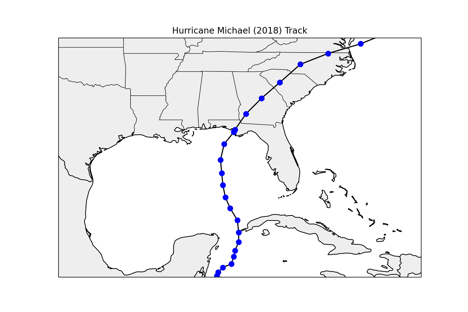
Now let’s make another plot of the Gulf of Mexico, with Hurricane Michael’s track colored in a solid black line, and individual observations plotted in blue dots:

# Create an instance of figure and axes
fig = plt.figure(figsize=(9,6),dpi=200)
ax = plt.axes(projection=proj) # We already defined "proj" earlier, so no need to redefine it
ax = plot_boundaries(ax)

# Append Tropycal functionality to this axes
ax = utils.add_tropycal(ax)

# Plot Hurricane Michael's track line
ax.plot_storm(storm, color='k', linewidth=1.5)

# Plot storm dots in blue
ax.plot_storm(storm, 'o', ms=8, mfc='blue', mec='none')

# Zoom in over the Gulf Coast
ax.set_extent([-100,-70,18,37])

# Add title
ax.set_title("Hurricane Michael (2018) Track")

Text(0.5, 1.0, 'Hurricane Michael (2018) Track')

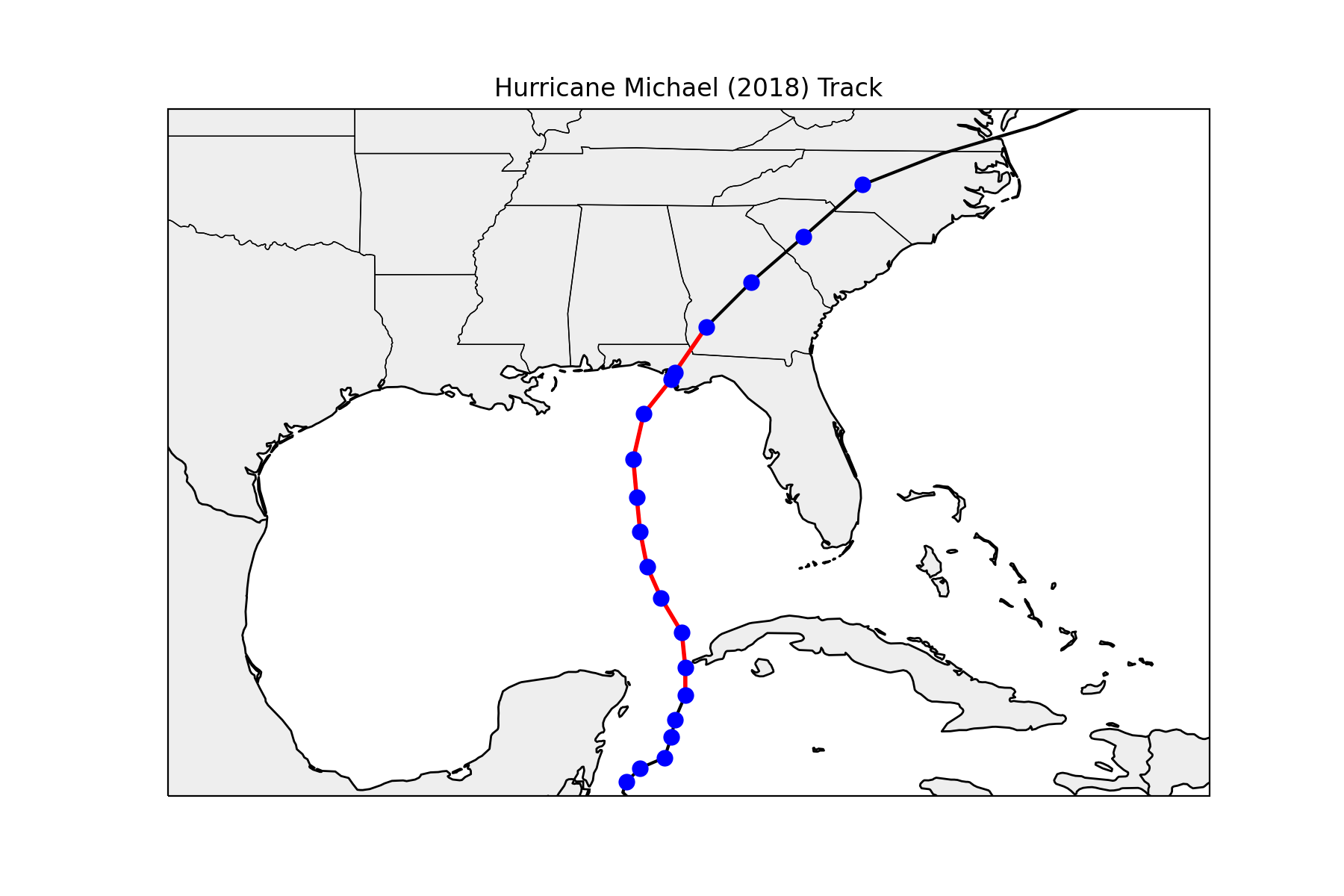
Let’s say we want to plot the portion where Michael was a hurricane in a different color, and where it was a non-tropical cyclone in a dashed black line. We can use subsetted Storm objects to accomplish this:

# Create an instance of figure and axes
fig = plt.figure(figsize=(9,6),dpi=200)
ax = plt.axes(projection=proj)
ax = plot_boundaries(ax)

# Append Tropycal functionality to this axes
ax = utils.add_tropycal(ax)

# Plot Hurricane Michael's track line
ax.plot_storm(storm, color='k', linewidth=1.5)

# ------------------------------------------------------------------

# Find all segments where Michael was a hurricane
def find_hurricane_segments(storm):

    # Create empty list to store data
    data = []

    # Loop over all times
    for i, i_time in enumerate(storm.time):
        if i == 0: continue

        # Find where hurricane segment began
        if storm.vmax[i] >= 64 and storm.vmax[i-1] < 64:
            data.append([i_time])

        # Find where hurricane segment ended
        elif storm.vmax[i] < 64 and storm.vmax[i-1] >= 64:
            data[-1].append(storm.time[i-1])

    #Return output
    return data

segments = find_hurricane_segments(storm)

# Subset the storm for each segment it was a hurricane, and plot a red line
for segment in segments:

    # Subset storm object
    storm_subset = storm.sel(time=(segment[0],segment[1]))

    # Plot segment in red
    ax.plot_storm(storm_subset, color='r', linewidth=2.0)

# ------------------------------------------------------------------

# Subset storm to the portion where it was a tropical cyclone
storm_tc = storm.sel(stormtype=['SD','SS','TD','TS','HU'])

# Plot storm dots only where Michael was a tropical cyclone
ax.plot_storm(storm_tc, 'o', ms=8, mfc='blue', mec='none')

# ------------------------------------------------------------------

# Zoom in over the Gulf Coast
ax.set_extent([-100,-70,18,37])

# Add title
ax.set_title("Hurricane Michael (2018) Track")

Text(0.5, 1.0, 'Hurricane Michael (2018) Track')

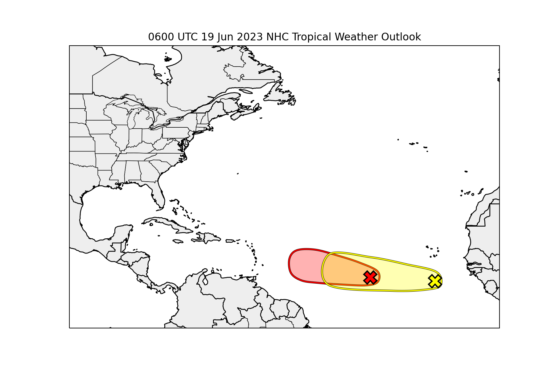
Plotting Tropical Weather Outlooks

We can also use Tropycal’s standalone plotting functionality to plot Tropical Weather Outlooks (TWOs) on an existing axes. First, let’s retrieve a TWO from a past date (e.g., 0600 UTC 19 June 2023):

requested_time = dt.datetime(2023,6,19,6)

two = utils.get_two_archive(time = requested_time)

Now we can plot this TWO on the axes with a North Atlantic projection. For this example we’ll use the default configuration, but the documentation offers more information on how to vary transparency, linewidth and zorder on the plot.

# Create an instance of figure and axes
fig = plt.figure(figsize=(9,6),dpi=200)
ax = plt.axes(projection=proj) # We already defined "proj" earlier, so no need to redefine it
ax = plot_boundaries(ax)

# Append Tropycal functionality to this axes
ax = utils.add_tropycal(ax)

# Plot TWO on this axes
ax.plot_two(two)

# Zoom in over the North Atlantic basin
ax.set_extent([-100,-10,0,50])

# Add title
ax.set_title(f"{requested_time.strftime('%H%M UTC %d %b %Y')} NHC Tropical Weather Outlook")

Possible issue encountered when converting Shape #0 to GeoJSON: Shapefile format requires that polygons contain at least one exterior ring, but the Shape was entirely made up of interior holes (defined by counter-clockwise orientation in the shapefile format). The rings were still included but were encoded as GeoJSON exterior rings instead of holes.
Possible issue encountered when converting Shape #0 to GeoJSON: Shapefile format requires that polygons contain at least one exterior ring, but the Shape was entirely made up of interior holes (defined by counter-clockwise orientation in the shapefile format). The rings were still included but were encoded as GeoJSON exterior rings instead of holes.

Text(0.5, 1.0, '0600 UTC 19 Jun 2023 NHC Tropical Weather Outlook')

Plotting Cone of Uncertainty

We can use this functionality to plot a cone of uncertainty generated from utils.generate_nhc_cone(). Let’s generate a cone of uncertainty for Hurricane Ian from 2022:

# Retrieve Hurricane Ian
storm = basin.get_storm(('ian',2022))

# Retrieve desired forecast
requested_time = dt.datetime(2022, 9, 27, 0)

#Create cone dict using default settings
cone = utils.generate_nhc_cone(
    forecast = storm.get_nhc_forecast_dict(requested_time),
    basin = 'north_atlantic',
    cone_days = 5,
    return_xarray = True,
)

We can now plot its track leading up to the requested time, and its cone of uncertainty and associated center line:

# Create an instance of figure and axes
fig = plt.figure(figsize=(9,6),dpi=200)
ax = plt.axes(projection=proj) # We already defined "proj" earlier, so no need to redefine it
ax = plot_boundaries(ax)

# Append Tropycal functionality to this axes
ax = utils.add_tropycal(ax)

# Plot observed storm track up to the requested time
storm_subset = storm.sel(time=(storm.time[0],requested_time))
ax.plot_storm(storm_subset, color='k', linestyle='dotted')

# Plot Hurricane Ian's forecast
ax.plot_cone(cone = cone,
             fillcolor = 'red',
             alpha = 0.3,
             plot_center_line = True,
             center_linecolor = 'blue',
             center_linestyle = 'dashed')

# Plot dot over Ian's location at this time
ax.plot(storm_subset.lon[-1], storm_subset.lat[-1], 'o',
        mfc='k', mec='none', ms=12, transform=ccrs.PlateCarree())

# Zoom in over the Gulf Coast
ax.set_extent([-100,-70,18,37])

# Add title
ax.set_title("Hurricane Ian (2022) NHC Forecast Cone", loc='left', fontsize=12)
ax.set_title(f"Forecast Issued: {requested_time.strftime('%H%M UTC %d %b %Y')}", loc='right', fontsize=10)

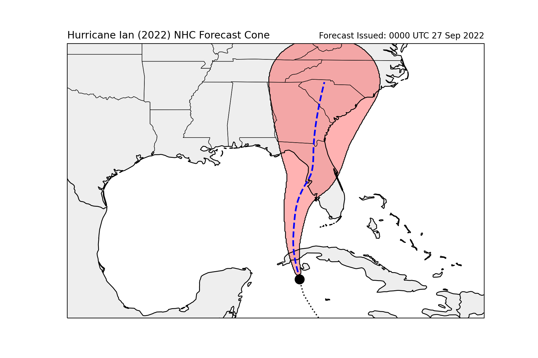
Text(1.0, 1.0, 'Forecast Issued: 0000 UTC 27 Sep 2022')