Customizing Storm Plots

This sample script illustrates how to leverage Tropycal’s plotting functionality to customize storm track plots.

import tropycal.tracks as tracks
import datetime as dt

Reading In HURTDAT2 Dataset

Let’s start with the HURDAT2 dataset by loading it into memory. By default, this reads in the HURDAT dataset from the National Hurricane Center (NHC) website, unless you specify a local file path using either atlantic_url for the North Atlantic basin on pacific_url for the East & Central Pacific basin.

HURDAT data is not available for the current year. To include the latest data up through today, the “include_btk” flag needs to be set to True, which reads in preliminary best track data from the NHC website. For this example, we’ll set this to False.

Let’s create an instance of a TrackDataset object, which will store the North Atlantic HURDAT2 dataset in memory. Once we have this we can use its methods for various types of analyses.

basin = tracks.TrackDataset(basin='north_atlantic',include_btk=False)

--> Starting to read in HURDAT2 data
--> Completed reading in HURDAT2 data (2.07 seconds)

Methods to Plot Storm Track

There are two primary methods to plot an individual storm track. The first two will use our TrackDataset instance, which contains the entire HURDATv2 database.

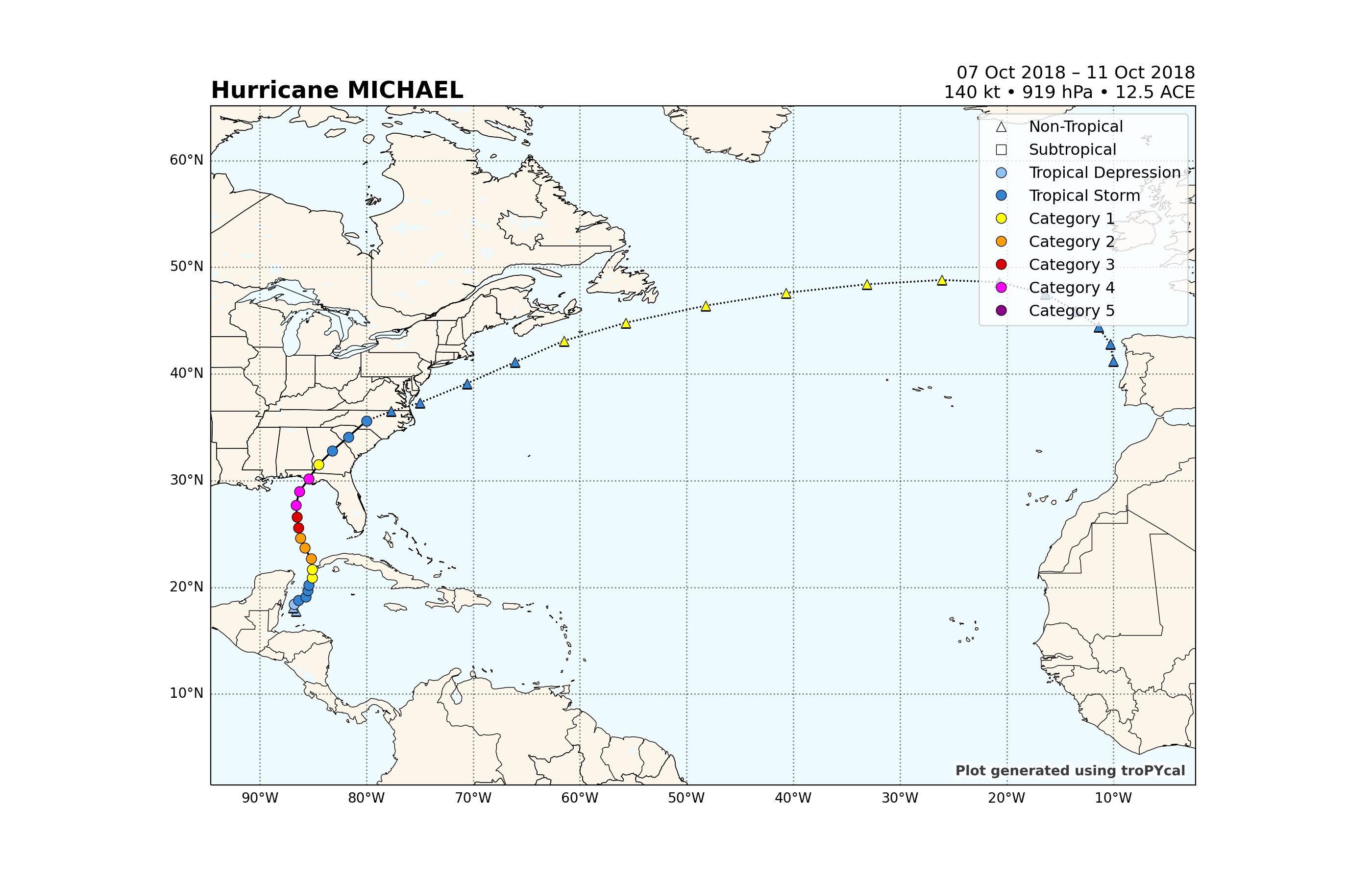
Let’s say we want to plot Hurricane Michael (2018). The first way we can do this is to use basin.plot_storm(), where the first argument is either a storm ID (e.g., "AL142018"), or a storm tuple (e.g., ("michael",2018)).

#Plot Hurricane Michael's track directly from the TrackDataset instance
basin.plot_storm(('michael',2018))

<GeoAxes: title={'left': 'Hurricane MICHAEL', 'right': '07 Oct 2018 – 11 Oct 2018\n140 kt • 919 hPa • 12.5 ACE'}>

The second method is to retrieve a Storm object from basin, and then plot from the Storm instance we just retrieved.

#Retrieve an instance of Storm for Hurricane Michael and store it in the variable "storm":
storm = basin.get_storm(('michael',2018))

#Plot the storm track for this Storm instance
storm.plot()

<GeoAxes: title={'left': 'Hurricane MICHAEL', 'right': '07 Oct 2018 – 11 Oct 2018\n140 kt • 919 hPa • 12.5 ACE'}>

Customizing Our Plot

This seems easy enough so far, right? Now let’s say we want to customize our plot. There’s multiple way we can customize this plot, detailed more thoroughly in the documentation. The code below shows some of these methods.

Hurricane Michael tracked quite far as an extratropical cyclone, but for this purpose we want to focus in on the portion where it was tropical. By default, plotting storms is set to domain='dynamic', which zooms in on the entire track. Let’s change this to a bounded region from 15N to 40N latitude, and from 105W to 65W longitude:

storm.plot(domain={'w':-105,'e':-65,'s':15,'n':40})

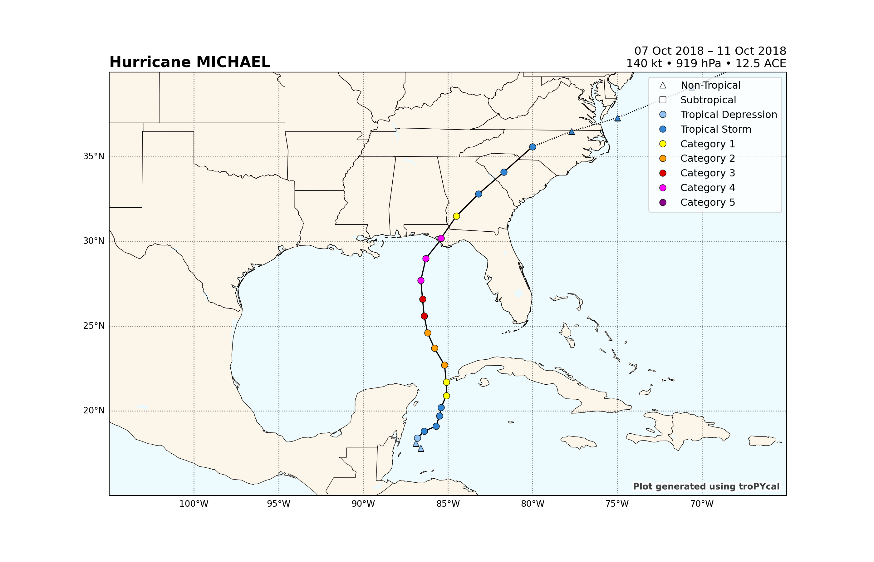
<GeoAxes: title={'left': 'Hurricane MICHAEL', 'right': '07 Oct 2018 – 11 Oct 2018\n140 kt • 919 hPa • 12.5 ACE'}>

This works for Michael, but it can get quite burdensome if we constantly have to hard-code this for every storm. Fortunately, we can simply use domain="dynamic_tropical", which zooms in only where the system was a tropical cyclone:

storm.plot(domain='dynamic_tropical')

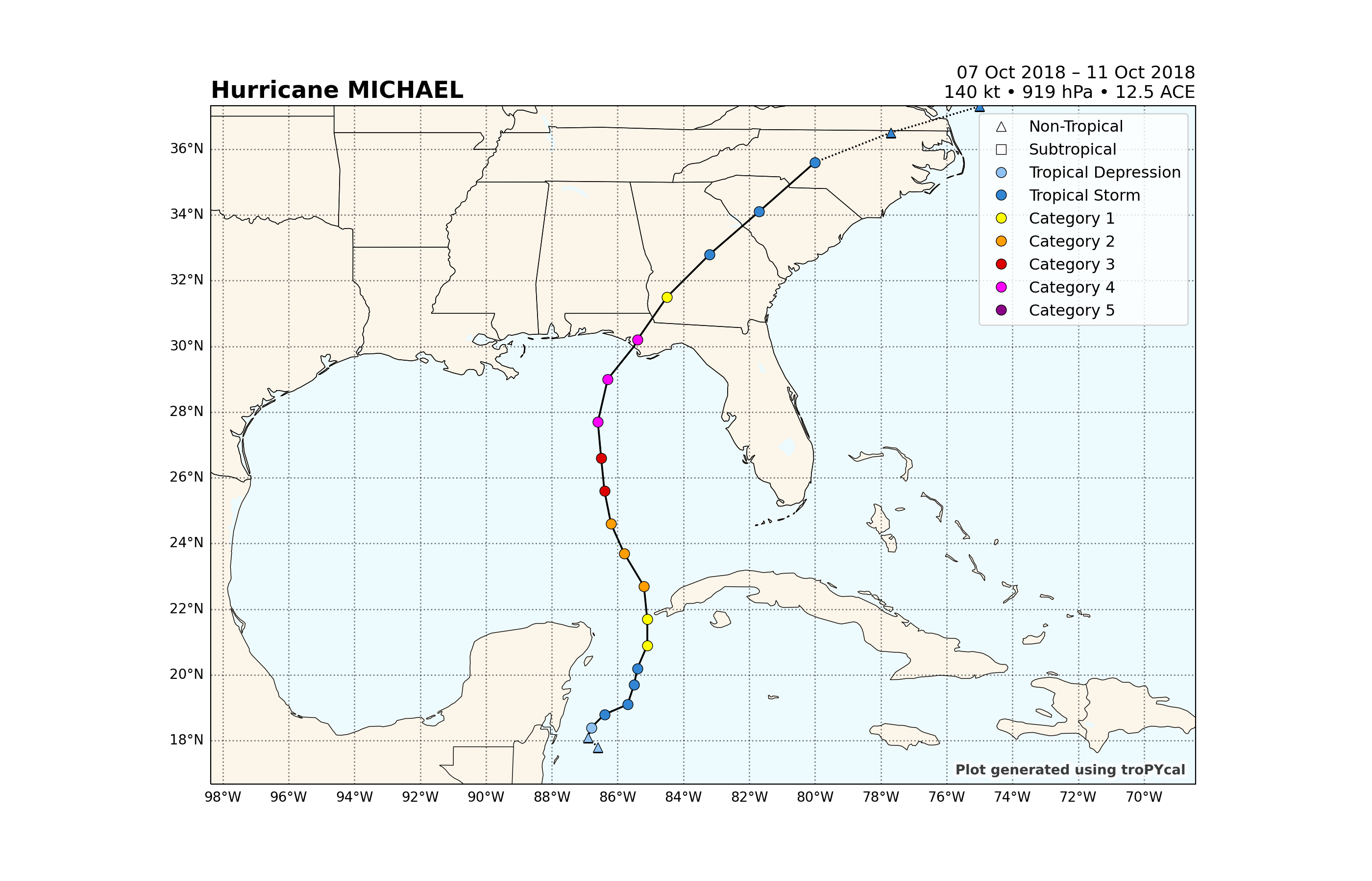
<GeoAxes: title={'left': 'Hurricane MICHAEL', 'right': '07 Oct 2018 – 11 Oct 2018\n140 kt • 919 hPa • 12.5 ACE'}>

Now let’s start to experiment with different coloring and line properties. Say we want to start off simple and color all dots blue with a larger marker size, and all lines red with a line width of 2.0. We can modify the prop keyword argument:

storm.plot(domain='dynamic_tropical',prop={'ms':10,'fillcolor':'blue','linecolor':'red','linewidth':2.0})

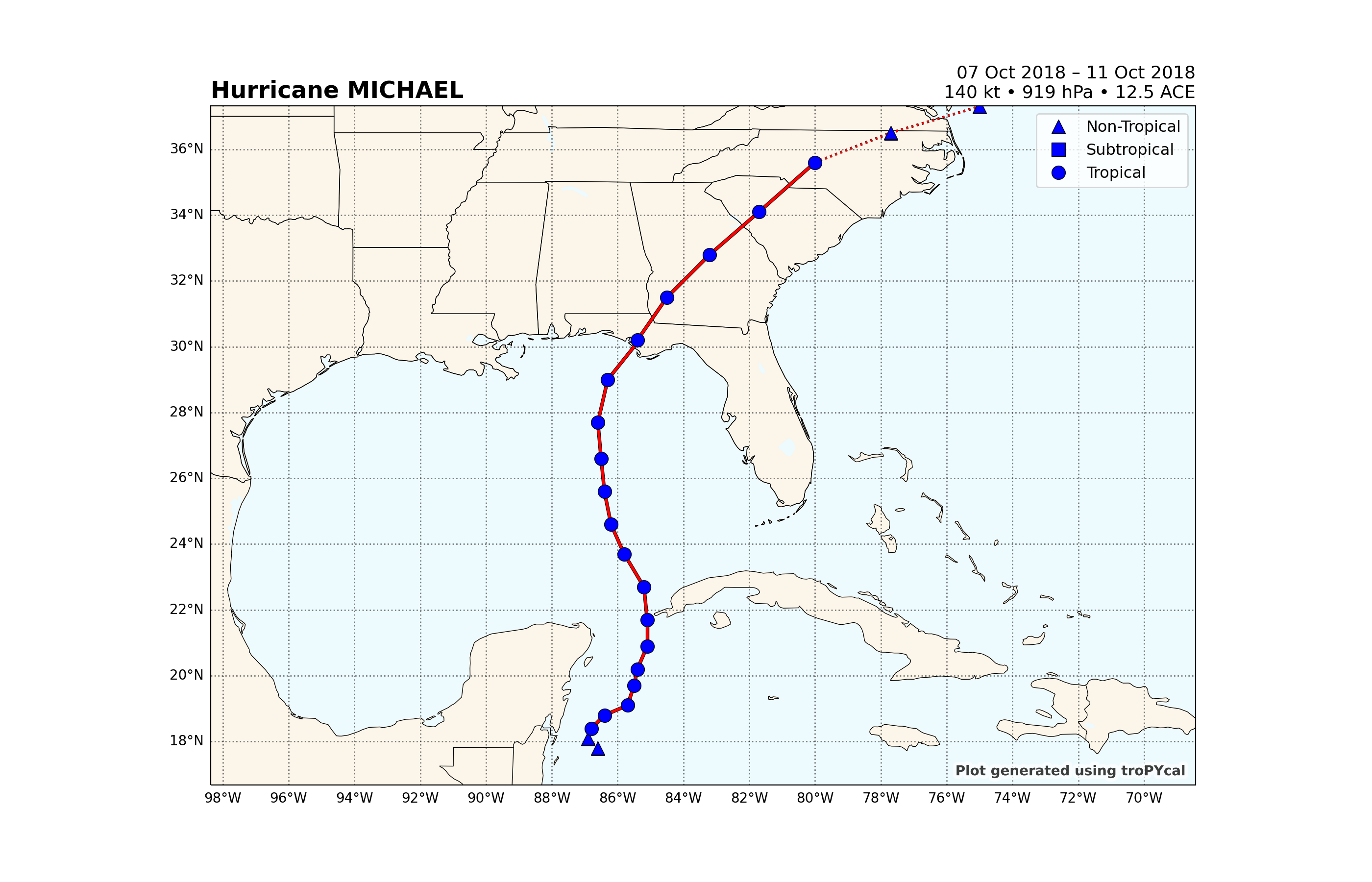
<GeoAxes: title={'left': 'Hurricane MICHAEL', 'right': '07 Oct 2018 – 11 Oct 2018\n140 kt • 919 hPa • 12.5 ACE'}>

By default, the dots are colored by the Saffir-Simpson Hurricane Wind Scale (SSHWS) category. This is because the default value for fillcolor is “category”. If we want to color the track line by category, and to not plot dots, we can do the following:

storm.plot(domain='dynamic_tropical',prop={'dots':False,'linecolor':'category','linewidth':3.0})

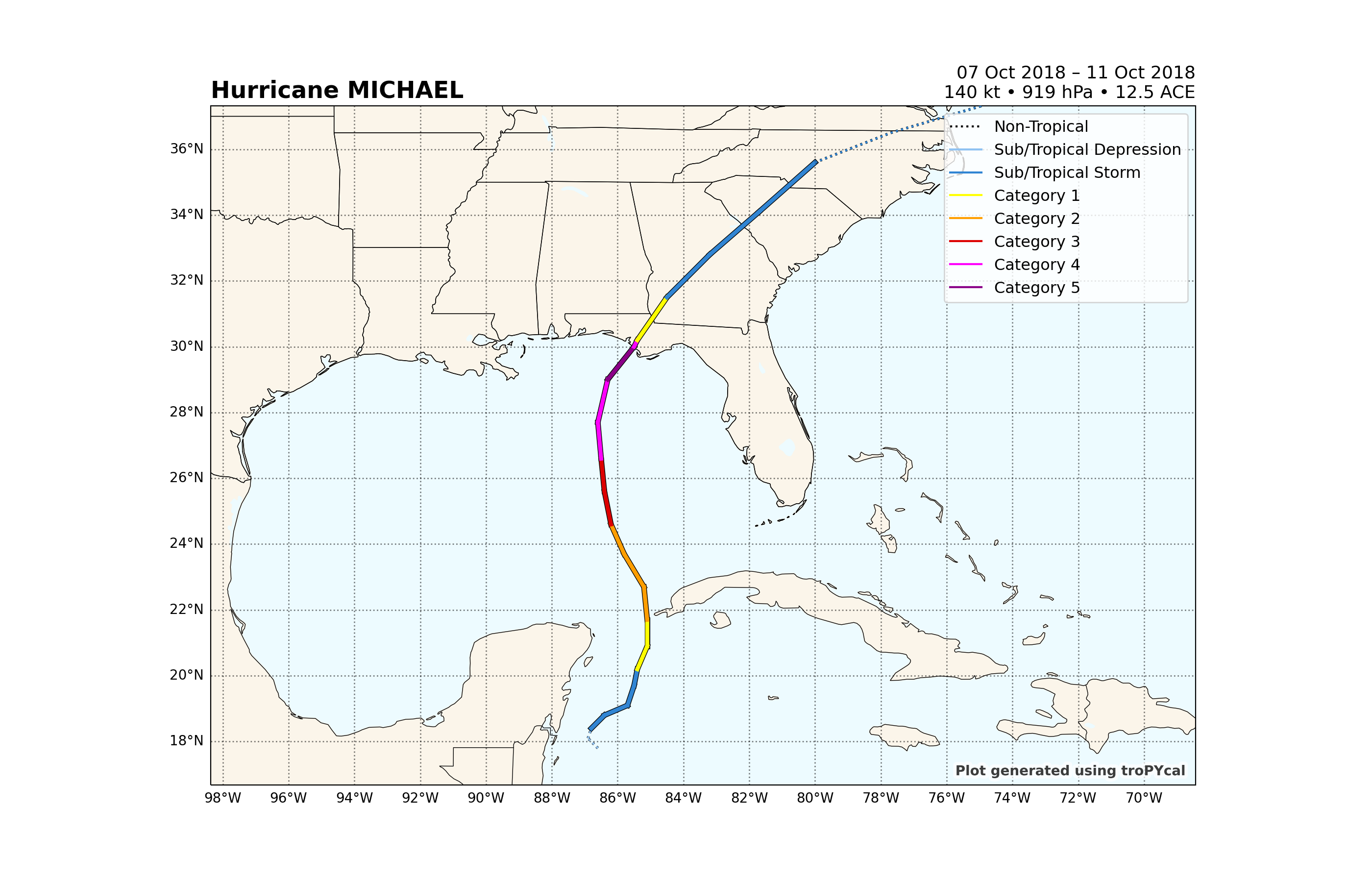
<GeoAxes: title={'left': 'Hurricane MICHAEL', 'right': '07 Oct 2018 – 11 Oct 2018\n140 kt • 919 hPa • 12.5 ACE'}>

We can also use other coloring options for the plot. For example, say we want to color the track line by maximum sustained wind (in knots) - we simply plug in “vmax” for linecolor. While not shown below, we can do the same for “mslp”.

storm.plot(domain='dynamic_tropical',prop={'dots':False,'linecolor':'vmax','linewidth':3.0})

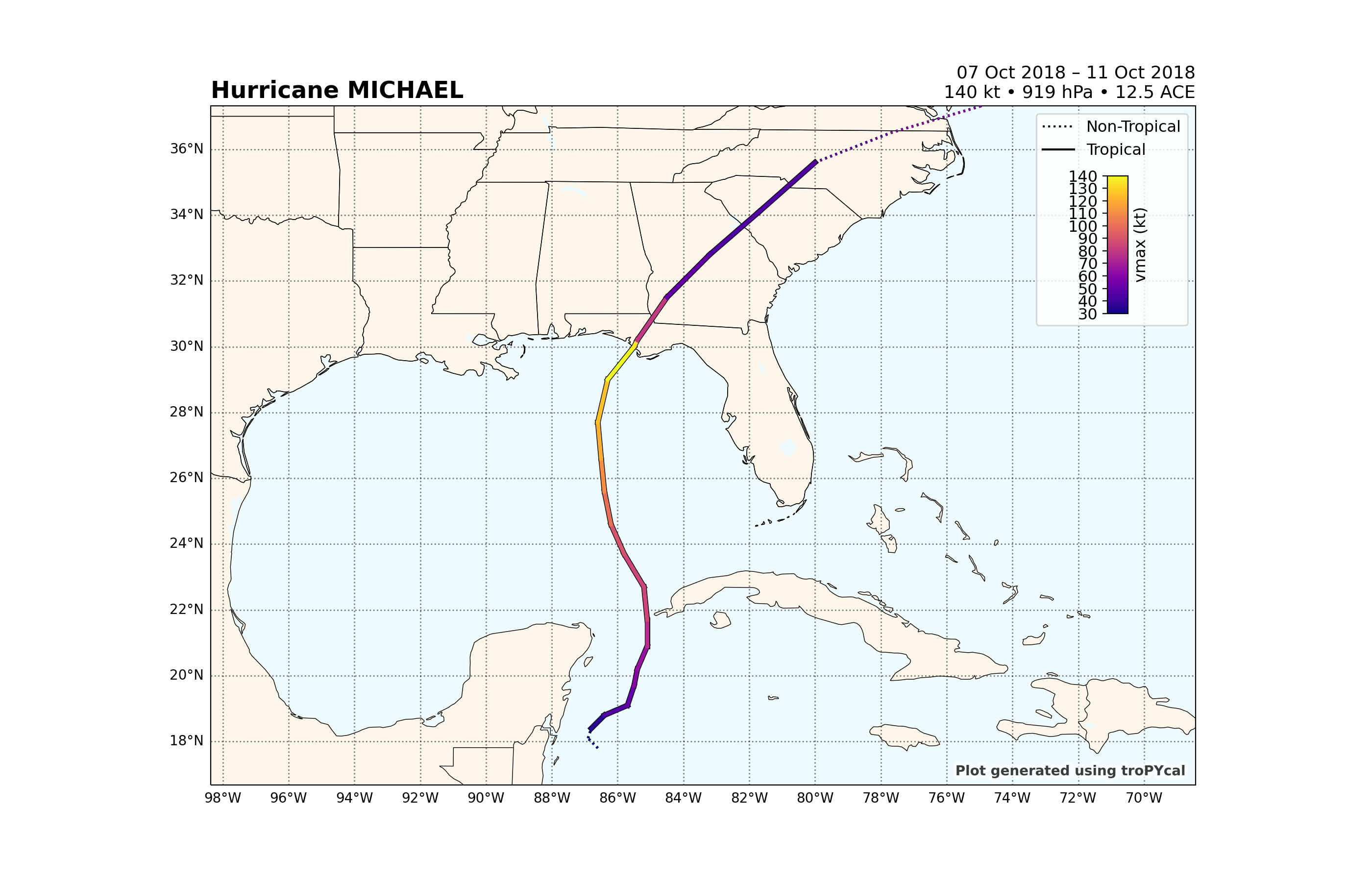
<GeoAxes: title={'left': 'Hurricane MICHAEL', 'right': '07 Oct 2018 – 11 Oct 2018\n140 kt • 919 hPa • 12.5 ACE'}>

Moving on to more complicated colorings, we can also color the line by change in sustained wind speed (“dvmax_dt”), and the forward motion of the cyclone (“speed”). For this, we have to use an interpolated Storm object, interpolating the data to hourly:

We’ll also use a custom colormap to make rapid intensification and rapid weakening stand out more clearly.

#Interpolate storm to hourly, and store as a new Storm object
storm_interpolated = storm.interp()

#Make a custom colormap, matching values to a color. These are then linearly interpolated when making the plot.
cmap = {-60:'violet',-30:'royalblue',-29.99:'dodgerblue',0:'w',29.99:'tomato',30:'firebrick',60:'violet'}

storm_interpolated.plot(domain='dynamic_tropical',prop={
    'dots' : False,
    'linecolor' : 'dvmax_dt',
    'linewidth' : 3.0,
    'cmap' : cmap,
    'levels' : (-61,61)
})

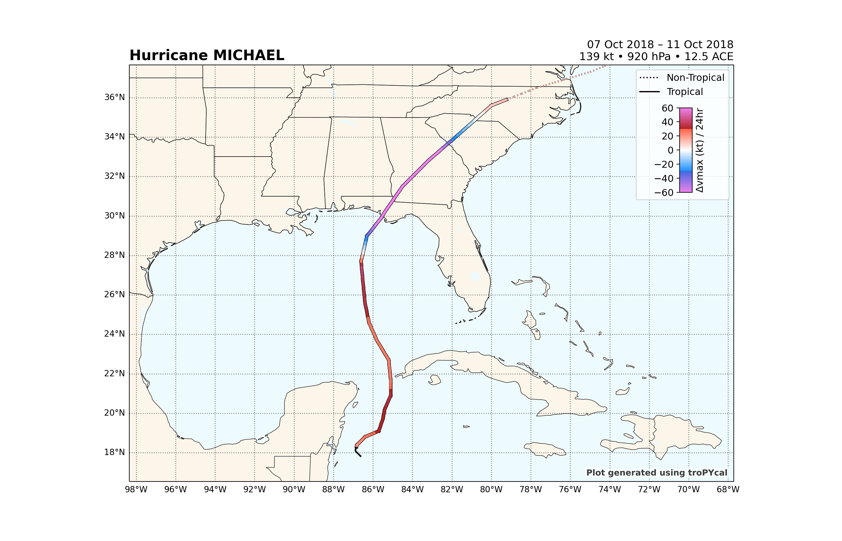
<GeoAxes: title={'left': 'Hurricane MICHAEL', 'right': '07 Oct 2018 – 11 Oct 2018\n139 kt • 920 hPa • 12.5 ACE'}>

Plotting Multiple Storms

We can also plot multiple storms in the same plot. For this, we’ll go back to our TrackDataset object, which has the ability to plot multiple storm tracks.

Let’s plot the four Category 5 hurricanes in the 2005 Atlantic Hurricane Season: Emily, Katrina, Rita and Wilma.

basin.plot_storms([('emily',2005),('katrina',2005),('rita',2005),('wilma',2005)])

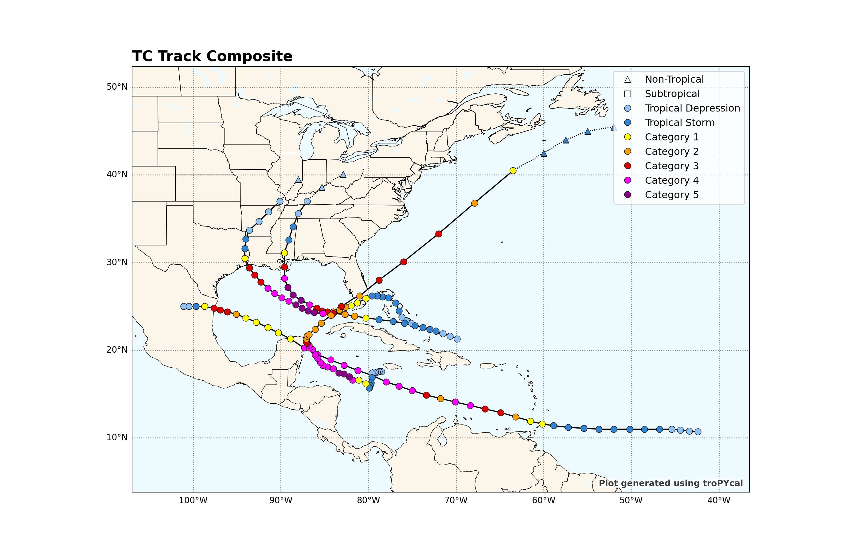
<GeoAxes: title={'left': 'TC Track Composite'}>

Using what we did earlier, let’s customize the plot to (1) not plot dots, (2) color lines by SSHWS category, (3) set linewidth to 3, and additionally label the storm names using 'plot_names':True.

basin.plot_storms([('emily',2005),('katrina',2005),('rita',2005),('wilma',2005)],
                  prop={'dots':False,'linecolor':'category','linewidth':3,'plot_names':True})

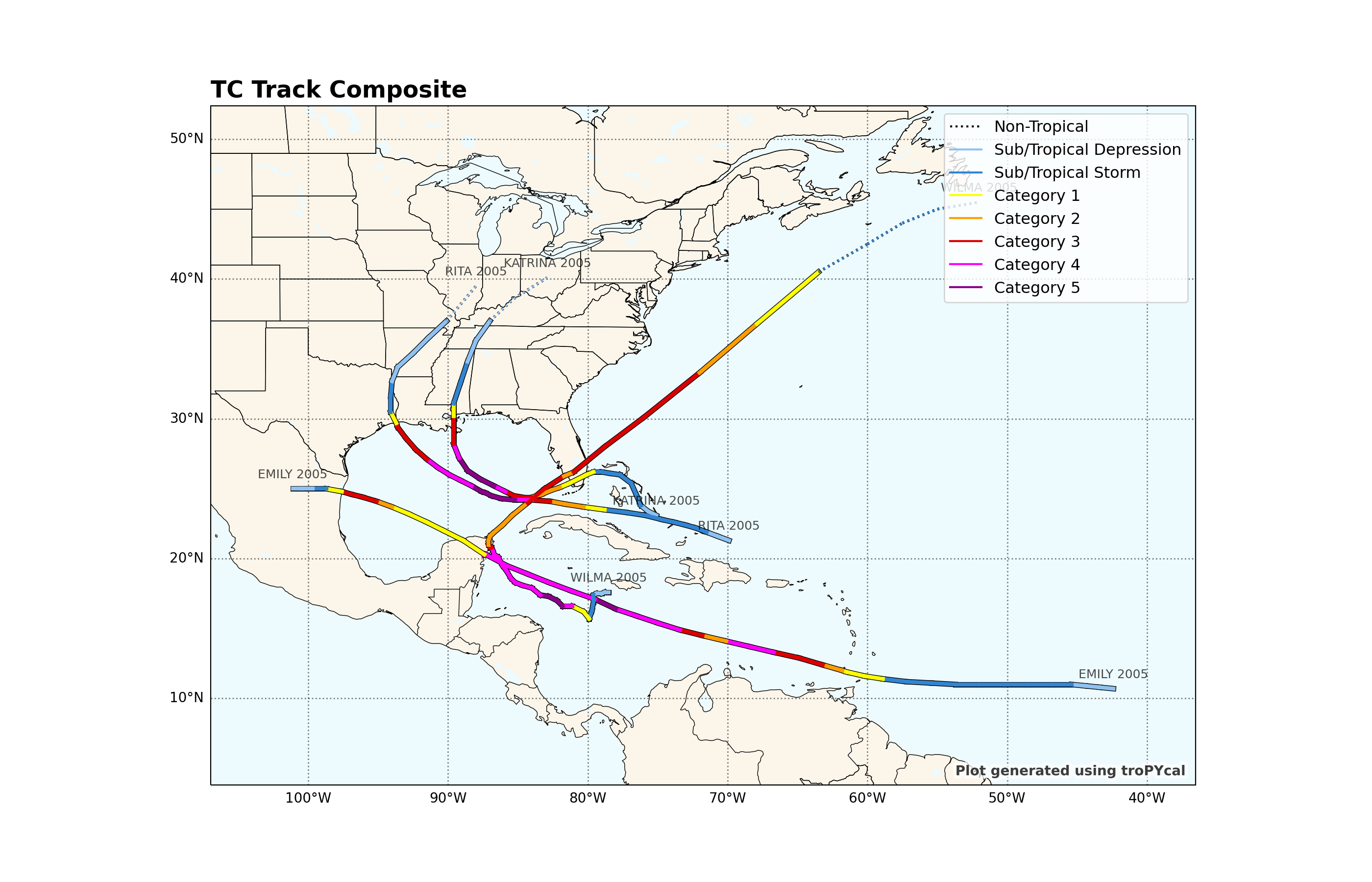
<GeoAxes: title={'left': 'TC Track Composite'}>