Reading SHIPS Data

This sample script illustrates how to leverage Tropycal’s SHIPS reading capability.

import json
import datetime as dt
import matplotlib.pyplot as plt
from tropycal import tracks

Reading In HURTDAT2 Dataset

Let’s start with the HURDAT2 dataset by loading it into memory. By default, this reads in the HURDAT dataset from the National Hurricane Center (NHC) website, unless you specify a local file path using either atlantic_url for the North Atlantic basin on pacific_url for the East & Central Pacific basin.

HURDAT data is not available for the current year. To include the latest data up through today, the “include_btk” flag needs to be set to True, which reads in preliminary best track data from the NHC website. For this example, we’ll set this to False.

Let’s create an instance of a TrackDataset object, which will store the North Atlantic HURDAT2 dataset in memory. Once we have this we can use its methods for various types of analyses.

basin = tracks.TrackDataset(basin='north_atlantic',include_btk=False)

--> Starting to read in HURDAT2 data
--> Completed reading in HURDAT2 data (1.66 seconds)

Reading in SHIPS data

SHIPS data can be read either using the standalone ships.Ships class by providing the SHIPS text data, or via Storm objects. The more conventional method is via Storm objects, as this automatically locates the SHIPS text files from UCAR’s online archive dating back to 2011.

Let’s retrieve an instance of Hurricane Ida from 2021 for our example:

storm = basin.get_storm(('ida',2021))

Next, let’s search for times where SHIPS forecasts are available:

available_times = storm.search_ships()

for time in available_times:
    print(time)

2021-08-26 12:00:00
2021-08-26 18:00:00
2021-08-27 00:00:00
2021-08-27 06:00:00
2021-08-27 12:00:00
2021-08-27 18:00:00
2021-08-28 00:00:00
2021-08-28 06:00:00
2021-08-28 12:00:00
2021-08-28 18:00:00
2021-08-29 00:00:00
2021-08-29 06:00:00
2021-08-29 12:00:00
2021-08-29 18:00:00
2021-08-30 00:00:00
2021-08-30 06:00:00
2021-08-30 12:00:00
2021-08-30 18:00:00

Now that we know what times are available, let’s use the SHIPS forecast from 1800 UTC 27 August 2021. The following line retrieves an instance of a Ships object and stores it in the variable ships:

ships = storm.get_ships(dt.datetime(2021, 8, 27, 18))

We now have a Ships object containing the forecast initialized at this time. Let’s peek at our Ships object:

print(ships)

<tropycal.ships.Ships>

Variables:
    fhr               (int) [0 .... 168]
    vmax_noland_kt    (int) [70 .... 55]
    vmax_land_kt      (int) [70 .... 27]
    vmax_lgem_kt      (int) [70 .... 27]
    storm_type        (str) [TROP .... TROP]
    shear_kt          (int) [11 .... 16]
    shear_adj_kt      (int) [-1 .... 0]
    shear_dir         (int) [216 .... 348]
    sst_c             (float) [29.5 .... 29.3]
    vmax_pot_kt       (int) [162 .... 156]
    200mb_temp_c      (float) [-52.8 .... -54.1]
    thetae_dev_c      (int) [9 .... 1]
    700_500_rh        (int) [64 .... 45]
    model_vortex_kt   (int) [17 .... 7]
    850mb_env_vort    (int) [47 .... 16]
    200mb_div         (int) [86 .... -35]
    700_850_tadv      (int) [8 .... -8]
    dist_land_km      (int) [98 .... -32]
    lat               (float) [21.6 .... nan]
    lon               (float) [-82.7 .... nan]
    storm_speed_kt    (int) [14 .... 7]
    heat_content      (int) [71 .... 4]

RI Probabilities:
    20kt/12hr:  61% (12.4x climo mean)
    25kt/24hr:  82% (7.5x climo mean)
    30kt/24hr:  76% (11.1x climo mean)
    35kt/24hr:  70% (17.9x climo mean)
    40kt/24hr:  53% (22.2x climo mean)
    45kt/36hr:  73% (15.8x climo mean)
    55kt/48hr:  47% (10.0x climo mean)
    65kt/72hr:  31% (5.9x climo mean)

Attributes:
    forecast_init:                 2021-08-27 18:00:00
    storm_name:                    IDA
    storm_bearing_deg:             325
    storm_motion_kt:               14
    max_wind_t-12_kt:              45
    steering_level_pres_hpa:       518
    steering_level_pres_mean_hpa:  620
    brightness_temp_stdev:         4.8
    brightness_temp_stdev_mean:    14.5
    pixels_below_-20c:             99.0
    pixels_below_-20c_mean:        65.0
    lat:                           21.6
    lon:                           -82.7

Retrieving Data

There’s a lot of data in this object, as SHIPS files provide a lot of variables over many forecast hours. If we want data only valid at a specific forecast hour, we can use the following method:

output_dict = ships.get_snapshot(hour=48)

# Format nicely for documentation purposes
print(json.dumps(output_dict, indent=4))

{
    "fhr": 48,
    "vmax_noland_kt": 121,
    "vmax_land_kt": 116,
    "vmax_lgem_kt": 127,
    "storm_type": "TROP",
    "shear_kt": 9,
    "shear_adj_kt": -5,
    "shear_dir": 263,
    "sst_c": 30.7,
    "vmax_pot_kt": 171,
    "200mb_temp_c": -51.8,
    "thetae_dev_c": 7,
    "700_500_rh": 73,
    "model_vortex_kt": 29,
    "850mb_env_vort": -8,
    "200mb_div": 41,
    "700_850_tadv": 6,
    "dist_land_km": 62,
    "lat": 28.6,
    "lon": -90.5,
    "storm_speed_kt": 8,
    "heat_content": 42
}

We can also fetch the rapid intensification probabilities that SHIPS provides:

output_dict = ships.get_ri_prob()

# Format nicely for documentation purposes
print(json.dumps(output_dict, indent=4))

{
    "20kt/12hr": {
        "probability": 61,
        "climo_mean": 4.9,
        "prob / climo": 12.4
    },
    "25kt/24hr": {
        "probability": 82,
        "climo_mean": 10.9,
        "prob / climo": 7.5
    },
    "30kt/24hr": {
        "probability": 76,
        "climo_mean": 6.8,
        "prob / climo": 11.1
    },
    "35kt/24hr": {
        "probability": 70,
        "climo_mean": 3.9,
        "prob / climo": 17.9
    },
    "40kt/24hr": {
        "probability": 53,
        "climo_mean": 2.4,
        "prob / climo": 22.2
    },
    "45kt/36hr": {
        "probability": 73,
        "climo_mean": 4.6,
        "prob / climo": 15.8
    },
    "55kt/48hr": {
        "probability": 47,
        "climo_mean": 4.7,
        "prob / climo": 10.0
    },
    "65kt/72hr": {
        "probability": 31,
        "climo_mean": 5.3,
        "prob / climo": 5.9
    }
}

Ships objects also allow us to convert data to other formats, such as xarray Datasets:

ds = ships.to_xarray()
print(ds)

<xarray.Dataset>
Dimensions:          (fhr: 17)
Coordinates:
  * fhr              (fhr) int64 0 6 12 18 24 36 48 ... 108 120 132 144 156 168
Data variables: (12/21)
    vmax_noland_kt   (fhr) int64 70 80 89 98 106 112 121 ... 74 66 61 58 57 55
    vmax_land_kt     (fhr) int64 70 67 83 92 100 107 116 ... 27 27 27 27 27 27
    vmax_lgem_kt     (fhr) int64 70 70 85 94 102 120 127 ... 27 27 27 27 27 27
    storm_type       (fhr) <U4 'TROP' 'TROP' 'TROP' ... 'TROP' 'TROP' 'TROP'
    shear_kt         (fhr) int64 11 13 11 8 7 17 9 16 11 19 12 25 20 24 12 18 16
    shear_adj_kt     (fhr) int64 -1 1 0 -3 -5 1 -5 5 1 1 3 0 3 -3 0 2 0
    ...               ...
    700_850_tadv     (fhr) int64 8 7 0 2 4 13 6 10 16 15 9 0 -3 -5 0 -10 -8
    dist_land_km     (fhr) int64 98 -18 126 268 410 ... -563 -461 -334 -200 -32
    lat              (fhr) float64 21.6 22.5 23.4 24.4 25.3 ... nan nan nan nan
    lon              (fhr) float64 -82.7 -83.8 -84.9 -85.8 ... nan nan nan nan
    storm_speed_kt   (fhr) int64 14 14 13 13 13 12 8 7 8 8 9 8 8 9 10 9 7
    heat_content     (fhr) int64 71 92 122 97 105 133 42 16 7 7 6 6 5 4 4 3 4
Attributes: (12/13)
    forecast_init:                 2021-08-27 18:00:00
    storm_name:                    IDA
    storm_bearing_deg:             325
    storm_motion_kt:               14
    max_wind_t-12_kt:              45
    steering_level_pres_hpa:       518
    ...                            ...
    brightness_temp_stdev:         4.8
    brightness_temp_stdev_mean:    14.5
    pixels_below_-20c:             99.0
    pixels_below_-20c_mean:        65.0
    lat:                           21.6
    lon:                           -82.7

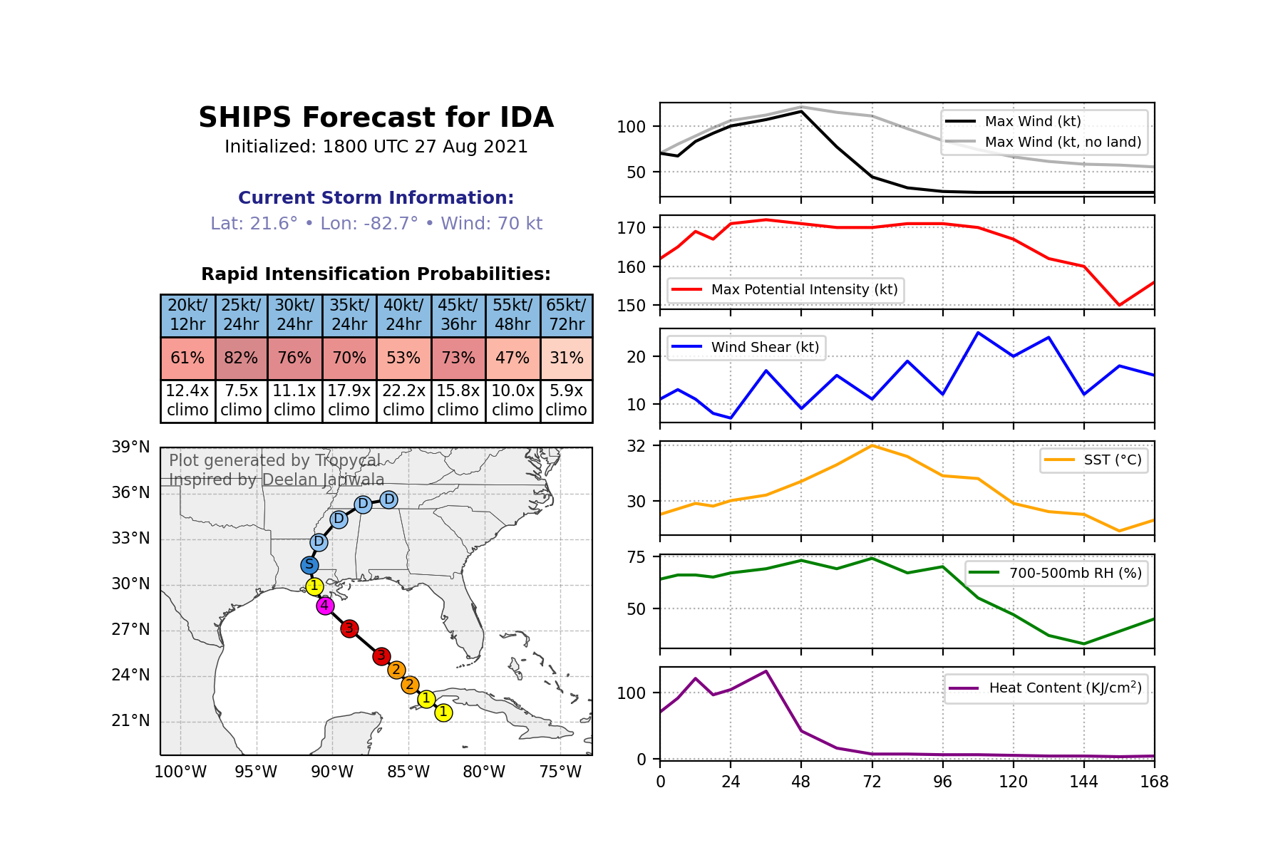
Visualizing Data

Tropycal’s Ships class comes with a built-in function to plot a basic summary of the SHIPS forecast and key diagnostics. We can use it as follows:

ships.plot_summary()

<Figure size 1800x1200 with 8 Axes>

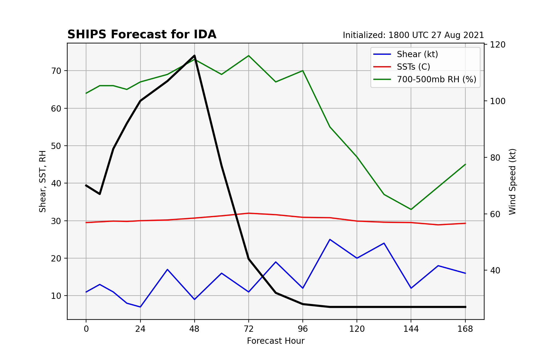
Let’s say we want to make a plot of several metrics that affect a storm’s intensity:

# Create figure
fig,ax = plt.subplots(figsize=(9,6), dpi=200)
ax.set_facecolor('#f6f6f6')
ax.grid()

# Plot variables
ax.plot(ships.fhr, ships.shear_kt, color='blue', label='Shear (kt)')
ax.plot(ships.fhr, ships.sst_c, color='red', label='SSTs (C)')
ax.plot(ships.fhr, ships['700_500_rh'], color='green', label='700-500mb RH (%)')
ax.set_ylabel('Shear, SST, RH')

# Add twin axes for wind speed
ax2 = ax.twinx()
ax2.plot(ships.fhr, ships.vmax_land_kt, color='k', linewidth=2.5)
ax2.set_ylabel('Wind Speed (kt)')

# Format and label x-axis
ax.set_xticks(range(0,ships.fhr[-1]+1,24))
ax.set_xlabel('Forecast Hour')

# Add legend and title
ax.legend()
ax.set_title(f"SHIPS Forecast for {ships.attrs['storm_name']}",
             loc='left', fontsize=14, fontweight='bold')
ax.set_title(f"Initialized: {ships.attrs['forecast_init'].strftime('%H%M UTC %d %b %Y')}",
             loc='right', fontsize=10)

Text(1.0, 1.0, 'Initialized: 1800 UTC 27 Aug 2021')